Registration required

The content you have requested is available only to registered visitors. Please complete the short form below (all fields are required).

  • 简体中文 简体中文 Chinese (Simplified) zh-hans
  • English English English en
Listen, Inc.
  • Products
    • AUDIO MEASUREMENT
    • System Overview
      • What Soundcheck Measures
      • SoundCheck for R&D
      • SoundCheck for Production
      • Innovation
    • SoundCheck Software
      • Making Measurements
      • Algorithm Highlights
      • Integration
      • What’s New?
      • Packages, Modules & Pricing
      • Support Contracts
    • Audio Measurement Interfaces
      • AudioConnect 2 (2 channel))
      • AmpConnect 621 (6/2 channels)
      • AudioConnect 8×8 (8 channel)
      • AudioConnect 6×2 (6/2 channel)
      • AmpConnect ISC (2 channel)
      • 3rd Party Audio Interfaces
    • Audio Testing Hardware
      • Microphones & Amplifiers
        • Measurement Microphones
        • Microphone Power
        • Audio Test Amplifier
      • Specialist Test Interfaces
        • Bluetooth Audio Measurement Interfaces
        • MEMS microphone Interfaces
        • DC Connect
      • Audio Test Accessories
        • Turntables
        • Halo Automotive 6-Mic Array
        • Automotive Audio Test Kit
        • The SCC-1 Ear Coupler
        • Other Measurement Transducers
        • Impedance Box
        • Calibrators
    • NOISE & VIBRATION MEASUREMENT
    • System Overview
    • NoiseCheck Software
    • Noise & Vibration Interfaces
    • Noise and Vibration Testing Hardware
  • Applications
    • Headphones & Headsets
    • Loudspeakers & Microspeakers
    • Microphones
    • Automotive
    • Communications
    • Smart Devices
    • Hearing Aids
    • Audio Electronics
  • Support
    • Get Support
    • User Documentation
    • Knowledgebase
    • Training
    • Sequences & Resources
    • Drivers
    • Register Product
    • Report a Bug / Request a Feature
  • Resources
    • ‘Sound Matters’ Blog: Audio Measurement Expertise
    • Test Sequences
    • Article Reprints
    • Published Papers
    • Technical Notes
    • Measurement Services
    • Useful References
  • News & Events
    • News
    • Events
  • About Listen
    • Listen, Inc.
    • Contact
    • Distributors & Reps
    • Careers
    • Privacy Policy
  • Menu Menu

Using SoundCheck’s Multi-Instrument FFT/RTA/Oscilloscope

October 14, 2025/in Blog, SoundCheck Tips Videos/by Julius Wijono

Visualize your measurements in real time with SoundCheck’s Multi-Instrument feature! In this video, we’ll show you how to use the integrated FFT analyzer, RTA, and oscilloscope to view synchronized time and frequency data, perform live calculations, and save custom instrument setups for quick recall.

Additional Resources for SoundCheck

Detailed explanations of how to use SoundCheck can be found in the SoundCheck manual.

Video Transcript: Using SoundCheck’s Multi-Instrument FFT/RTA/Oscilloscope

SoundCheck features a multi-channel Real Time spectrum analyzer, FFT Spectrum analyzer and Oscilloscope integrated into a single “multi-instrument”. This lets you view any number of live waveforms simultaneously, and results can be time-synchronized across the three instruments to simultaneously display parameters in both the time and frequency domain. Let’s check it out.

All three instruments can be opened from the instrument menu or with keyboard shortcuts which opens them with their default settings. Let’s open the FFT Spectrum analyzer. 

On the left is the control panel and next to it is the graph where the live curves are displayed. Live curves are also shown in the Memory List and identified with a green dot. The multi instrument graph is identified by its white shading around the plot area but otherwise, it has the same functions as the standard graphs used in SoundCheck display steps.

The acquisition controls are at the top of the control panel. The Record and Stop buttons are used to start and stop measurements, and when the instrument is in linear mode, the Continue button resumes the previous linear measurement and continues until the Start button is next used. The Add button lets us add new instruments, calculations, graphs and triggers to the multi instrument.

Let’s first open up the FFT Spectrum Analyzer and look at some of the analysis options for stationary signals such as sinewaves.

I’m outputting a 1 kHz tone at 2 Vrms from the signal generator. On the Multi-instrument graph, we can clearly see the fundamental and the 2nd and 3rd harmonics. Let’s drop a cursor on the fundamental using the snap to max function, enable the harmonic cursor and by exposing the advanced graph controls, we can get a real time readout of the cursor frequency, level and the THD of the fundamental. 

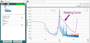
Now, let’s add a calculation, in this case a real-time masking curve which will show us how our dominant fundamental tone is masking other stationary signals. The masking curve suggests that all of the harmonics are below the threshold of hearing but as we increase the signal level, they get closer to being audible.  

By adding a second signal generator, we can view intermodulation products. One generator is set to 340 Hz and the other to  7 kHz with a 4:1 amplitude ratio between the two signals. With these settings, we can clearly see the intermodulation products around the 7 kHz tone.

I can save any virtual instrument configuration for later recall from the instruments menu. Let’s just ‘close all’ to close all my windows. And now I can re-open it without having to reopen and configure all of the individual instruments again. 

Let’s switch over to a saved configuration with the RTA and signal generator and look at some of the other calculation options. The Multi-Instrument graph supports both live curves from the RTA and static curves from the memory list, and can use them both in a calculation. 

Here, I’m sending a Pink Noise stimulus to the device under test and I want to compare its RTA spectrum to a target response curve, which is already in the Memory List.  I can  just drag the target curve over from the Memory List to display it on the live graph. Now, I add a calculation for dB subtraction where the live RTA curve is Operand A and the Target Curve from the Memory List is Operand B. This generates a real time difference curve on my live graph and I can name it something more descriptive. 

Another useful RTA calculation is Power Averaging.  Let’s add a couple of RTA’s to the current configuration and assign each a unique microphone signal path.  Notice how, when I add RTAs, they inherit the properties of the original RTA so all I have to do is update the Signal Path assignment. Now I can add the Power Average calculation, select all three microphones and we have the Power Average of the three microphones. Live curves can always be saved to the Memory List by clicking the Save to Memory button. Once there, they can be displayed on other graphs or saved to disc. Other available calculations include Maximum, Minimum and dB addition.

Let’s take a look at the oscilloscope. I’ll open a saved virtual instrument that is configured with two oscilloscopes, monitoring two different input signal paths. The oscilloscope control panel lets us set the data name, signal path selection, time base and measurement mode.  The measuring indicator is bright green when the instrument is active and dark green when stopped.

Now let’s pause the signal generators and add a trigger.  Our trigger level is set relative to the signal’s peak level using either linear or logarithmic scaling. Slope selection lets the user decide whether the scope will trigger on the first positive or negative portion of the incoming signal and offset allows you to define the amount of time that the Acquired Signal is shifted, relative to the point at which it is triggered.

The trigger level is set to 300 millivolts on Direct Input 5 so let’s start the signal generators and increase the signal level, and once we exceed the trigger threshold we can see how the scope starts running and when the signal goes below the trigger threshold it stops.

I hope you’ve learned a few things about the multi-instrument from this quick tip. Try it out for yourself, and don’t forget to check the user manual for more details.

https://www.listeninc.com/wp/media/2025/10/Multi-Instruments-Blog-TN.png 1080 1080 Julius Wijono https://www.listeninc.com/wp/media/logo.png Julius Wijono2025-10-14 06:00:452026-08-27 14:08:37Using SoundCheck’s Multi-Instrument FFT/RTA/Oscilloscope

Trigger Options for Open Loop Testing

September 30, 2025/in Blog/by Julius Wijono

Improve open loop audio testing with SoundCheck’s trigger options. In this video, we’ll show you how to configure level, frequency, and cross-correlation triggers to ensure accurate playback and recording in asynchronous test setups.

Additional Resources for SoundCheck

Detailed explanations of how to use SoundCheck can be found in the SoundCheck manual.

Video Transcript: Trigger Options for Open Loop Testing

Open-loop testing is used when the device under test, such as a microspeaker in a phone or tablet, cannot be physically connected to the test system, so playback and recording are asynchronous. 

Typically, we load the stimulus signal onto the device under test, and play it back during the sequence run, capturing it with a record only acquisition step.

We need to incorporate a trigger into the acquisition step  so that SoundCheck knows when to start recording.

SoundCheck has three different trigger options – let’s take a look at how to use them.

Whichever trigger you use, first you need to create your test stimulus and save it as a wav file. In this case, we’ll take our stepped sine sweep from 20 kHz to 100 Hz and save it to a wav file. You could even add an autosave step to your sequence to perform this function.

Now let’s add a trigger. There are three trigger options available in the Record Only acquisition step – a level trigger, a level and frequency trigger and a level and cross-correlation trigger.

The level trigger step is our oldest and simplest method. SoundCheck just waits until the trigger level is exceeded on the selected input signal path, then records for the duration entered into the time field, which should be set to slightly longer than the stimulus duration. A small offset value can be applied to shift the recorded time waveform relative to the trigger time. In this case we add 100 ms to the start of the recorded time waveform prior to the trigger time. The timeout value is the amount of time that the step will wait for a trigger event before stopping.

Let’s run this.

Now that we have the Recorded Time Waveform in the Memory List, we can continue with analysis, post processing and other steps the same way as with a typical closed loop sequence.

If no trigger occurs before the Timeout value, the step produces a failed verdict in the sequence editor. We can configure the step to Halt on Fail, or to jump to an Operator Message prompting the operator to test again 

Simple level triggers are susceptible to false triggering – background noise, rather than the trigger tone might start the recording. Let me show you. I’ll run the sequence again while creating some noise, and you can see here, I triggered the recording with my clapping and we haven’t captured meaningful data.

Our second trigger option was designed to overcome such situations. The level and frequency trigger requires not only a level threshold to be exceeded but also a sine wave to be detected. This is more robust and less susceptible to errors due to background noise than the simple level trigger.

For this trigger, we create a compound stimulus. Here, our stimulus is a stepped sine sweep and we’ve configured the trigger tone as a 250ms 1 kHz sinewave. I’ve placed 100 ms of silence between the two components – that’s not a requirement. We set both the trigger tone and the silence to “Do not analyze” so we’re only analyzing the sweep portion of the recorded time waveform. 

Let’s run it. You can hear the trigger tone at the start, and you can see it on the recorded waveform here. And you can see, it’s analyzed just the sweep part of the stimulus to give us our results.

Although the level and frequency trigger is adequate for most purposes, it can occasionally register false triggers in noisy production applications where a neighboring line might be playing a similar trigger or sweeping through the trigger frequency. The cross-correlation trigger overcomes this by using a log sweep, or chirp, instead of a fixed tone trigger. You need the Time Selective Response module enabled on your SoundCheck license to use this option.  

(action: Help > Optional Modules and close then open STI editor)

In the cross correlation trigger, our fixed trigger tone is replaced by  a log sweep or “chirp”. The chirp should have a duration of 50 to 200 ms and have a frequency range of at least one octave, occurring within the passband of the device under test.

Now let’s select the Trigger type and the compound stimulus from the dropdown list in the acquisition step.

Let’s run it. You can see our log chirp here, and our stimulus, and of course our results.

That’s a quick demonstration of how to configure SoundCheck’s trigger options. You can find more detailed instructions in the user manual.

https://www.listeninc.com/wp/media/2025/09/Open-Loop-Blog-TN.png 1080 1080 Julius Wijono https://www.listeninc.com/wp/media/logo.png Julius Wijono2025-09-30 11:15:352026-08-27 13:50:30Trigger Options for Open Loop Testing

Why Headphone Target Curves and THD Don’t Tell the Whole Story

September 29, 2025/in Audio Measurement Musings, Blog/by Julius Wijono

Introduction

After weeks of measuring, presenting, and debating headphones at events including the AES International Conference on Headphone Technology and xMEMS Live Asia, one thing is clear: headphone specifications rarely tell the whole story. Despite endless measurements, a lack of standards means there’s little consistency in the way frequency response, sensitivity, and THD are measured between manufacturers, making results nearly impossible to compare.


Why Frequency Response Specs Mislead

Frequency response measurements are hard to compare as most include the unique response of the ear simulator, yet it is rarely specified what simulator was used. Similarly, test level, corresponding sound pressure level, and the number of times the headphones were repositioned on the ear simulator and averaged is rarely stated. A clearer picture would come from showing frequency responses from several measurements to demonstrate how strongly the responses shift due to ear seal leaks and high frequency directional characteristics when the headphone is repositioned.

There would also be value in sharing individual harmonic curves so it’s clear how much of the THD is even versus odd order harmonics. This information reveals a lot about the type of distortion, cause and audibility. Specifications should also state whether measurements were made with ANC on or off, and wired or via Bluetooth connection.


The Problem with Target Curves

There was a lot of talk about target response curves at the AES Headphone Conference – unsurprising since Dr. Sean Olive was a keynote speaker. The legendary Harman Target Curve gained widespread recognition as the first widely-shared target curve based on listener preference using many subjects. It is understandable why this is a preferential design target over a diffuse field correction curve, which it is often compared to. That said, the diffuse field correction curve was designed as a reference curve, not a design target, so it’s not really comparing like-for-like. 

Target curves also have other limitations. Since a target curve is simply an ideal targeted frequency response, as with headphone frequency responses, information is rarely provided on the specific ear simulator used to develop the curve, making it challenging to reliably compare your own device to the target. The original Harman target curve was measured on a modified GRAS 43AG ear simulator with a custom pinna. This makes any comparison imperfect, since any other coupler will introduce its own signature. 

Target curves differ for in-ear and over-the-ear headphones, and although they are based on large amounts of empirical data, they are by definition, an average, and not specifically attuned to any one particular person. Furthermore, a specific target curve is not universally aspirational. For example, the gaming industry places more emphasis on factors such as spatial cues, bass, or clarity for voice than the frequency response that is ideal for listening to music.

Target curves are also one-dimensional, ignoring factors such as phase matching, distortion, time variance due to signal processing (such as that found in ANC), and other factors that contribute to listener perception.

The onboard DSP now available for headphones means that the natural progression of a target curve based on many people is a customized target curve. There were several papers at the conference, such as those by Nielsen and Hamasaki that addressed the evolution of customized target curves based on auditory models. This allows frequency response to be customized based on the listener’s ears,  but how then is that presented in a headphone specification? How does an independent reviewer even describe the sound quality, when each person will configure it differently?


ANC Headphones: Quieter but not always better

Active noise cancellation is another area where specifications do not fully represent listener experience. Manufacturers boast about noise reduction levels but rarely disclose how it is measured and how ANC affects the sound quality. Conventional measurements such as THD usually demonstrate that ANC reduces distortion, yet most audiophiles claim the opposite. In my paper “Active Noise Cancellation Distortion in Headphones” at the AES conference, I demonstrated that although THD is indeed reduced when ANC is activated, this measurement alone is an incomplete picture. Time domain analysis reveals time and phase variance showing where perhaps the experience of poorer sound quality comes from. Surprisingly, the best correlation to listener perception was found with the POLQA algorithm – a communications quality algorithm that is certainly not designed for measuring headphone performance! Clearly more work is needed to arrive at a similar measurement method that truly captures the effects of active noise cancellation in a way that correlates well with human hearing.

Ironically, although R&D engineers struggle with producing headphone specs that correlate to listener experience, we’ve made significant headway with perceptual production line test methods that align well with human hearing to identify manufacturing defects such as perceptual rub & buzz and perceptual transient distortion detection. 


Why Conventional THD fails for headphone measurements

A couple of weeks later, I presented at xMEMS Asia live events in Taipei and Shenzhen, where I talked about small drivers being used in headphones and wearables such as smart glasses and smart watches. This time I was addressing a specific issue with the way many people measure loudspeaker THD. 

Conventionally, harmonic distortion is compared to the fundamental at the stimulus frequency. This is not totally accurate as linear distortion is superimposed on the non-linear distortion. This often goes un-noticed in conventional speakers where the highest distortion is usually at low frequencies near resonance, and the fundamental response is typically fairly flat since it is not measured with an ear simulator. The target response for headphones, however, is not flat and their fundamental response influences their harmonic responses. 

Conventional THD measurements are also a poor choice for piezo-MEMS speakers. These tend to be very linear at low frequencies, exhibiting distortion peaks at higher frequencies above 5kHz. For such devices, distortion that lies outside the audible range can be misrepresented as audible when referenced to the fundamental at the stimulus frequency, creating a misleading picture that doesn’t match perception.

Since 1993 I have been promoting the use of frequency normalized distortion measurements. With frequency normalized distortion, the harmonic distortion is plotted at its measured frequency and compared to the fundamental response at the same frequency before plotting difference at the stimulus frequency which separates non-linear distortion from linear distortion. When piezo-MEMS speakers are measured using this method, it becomes clear that the higher distortion is just a consequence of their linear response or rising sensitivity versus frequency which is equalized to be flatter as part of the product design. It also makes resonances far clearer, allowing their effects to be mitigated, for example, by damping.

With the explosion in the use of MEMS speakers for headphones, hearing aids and wearables, I suspect that normalized distortion will at last become more widely accepted as the best way to measure THD. After all, accurate measurements are the key to good product design.


Closing the Gap Between Specs and Perception

So where does this leave us with headphone and headphone component measurements? 

If we want to be able to tell what a headphone sounds like from its specifications, the industry needs well-documented standardized tests such as IEC 60268-7 and measurement methods that go far beyond frequency response and THD. As these devices become more feature-rich with onboard DSP, ANC, custom response profiles and more, the industry must develop and standardize new measurement methods that correlate with human perception. 

Until then, we’ll just have to rely on the subjective opinion of the many reviewers out there, together with the objective measurements that they have made. At least when review sites make objective measurements, they use consistent equipment, making results comparable, even if they don’t align with manufacturer specifications.


  1. Temme, S. 1993 March 16-19. How to Graph Distortion Measurements. 94th AES Conference, Berlin, Germany.
  2. Temme, S. 2025 Aug 27-19. Active Noise Cancellation Distortion in Headphones. AES International Conference on Headphone Technology. Espoo, Finland.
https://www.listeninc.com/wp/media/2025/09/Steve_pres_cropped.jpg 814 582 Julius Wijono https://www.listeninc.com/wp/media/logo.png Julius Wijono2025-09-29 17:02:062025-11-21 11:36:22Why Headphone Target Curves and THD Don’t Tell the Whole Story

SoundCheck Sequence Editor Secrets

September 16, 2025/in Blog, SoundCheck Tips Videos/by Julius Wijono

Speed up your SoundCheck sequence development with hidden Sequence Editor features. In this video, we’ll show you secret tips for editing, debugging, and reusing steps to streamline sequence development.

Additional Resources for SoundCheck

Detailed explanations of how to use SoundCheck can be found in the SoundCheck manual.

Video Transcript: SoundCheck Sequence Editor Secrets

In this short video, I’m going to show you how to speed up your sequence development with some of the hidden features in SoundCheck’s powerful sequence editor. 

The sequence editor can be opened from the Setup menu or with the Ctrl + Q keyboard shortcut.

On the left side is our template library. You can drag the divider to re-size it, or click the divider to show or hide elements.

Step templates are grouped by category, and you can click on the expansion buttons to expand or contract them. You can right click on the category name to create new templates or import them from other versions of SoundCheck. Existing templates can also be edited, renamed or deleted. All sequences located in the folder of the active sequence are listed in the sequence template group.

The right side of the editor contains the active sequence.  The configuration menu at the top is where you set the default behavior for when the sequence opens, starts and runs, and set the path to any instruction files. There’s also a comment field where you can enter notes about the sequence.

The Sequence Parameters table is used to create Memory List placeholders which can be filled via external control using the MemoryList.set TCP/IP command. 

Lastly, the Metadata table is used to configure the sequence’s Metadata parameters.

Expanding a step shows you what data is coming in and out of the step. Steps are added to a sequence by dragging from the template library and dropping at the desired location. They can be configured as desired. A step or groups of steps can be moved within a sequence using drag and drop.

Now let’s take a look at the features in the right click menu.

Right clicking > Configure Step lets you configure step logic such as looping and jumping, as well as adding breakpoints and comment lines.

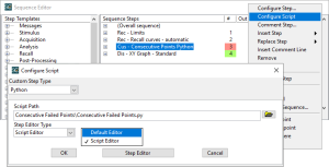
The configure Script option is only active for custom steps, where the script configuration window offers access to the LabView and Python options as well as the custom step editor

Commenting lets you enter descriptive text to help others understand what’s going on, step by step, and it’s a very useful feature, especially where your sequences are long or complex. In this sequence we’ve used comment steps to describe individual step functions and comment lines to explain where different river measurements take place for a 3-way loudspeaker.

Insert and Replace step are self explanatory. Insert is an alternative to drag and drop, and ‘replace’ replaces an existing step with a new step from the template library.

Copy and paste is a new feature we introduced in SC23. You can either use the right click menu or control+C control+V keyboard shortcuts.

Remove – as the same suggests, it removes or deletes the step 

Rename – lets you change the default name to something more descriptive

Undo – lets you undo the last several actions including inserting, removing and editing steps

Expand/Collapse all is a global command that expands and collapses all steps in the sequence. and is useful for determining where certain inputs and outputs are happening during the sequence run.

We also have some powerful tools for sequence debugging and editing.

Breakpoints are really useful when you’re working on long or complex sequences. You can define points in the sequence where it breaks from running, then use the toolbar buttons to either advance to the next step or the end of the section. This lets you isolate and run  small parts of the sequence without having to run the entire sequence. Here I’ll add 4 breakpoints. Now I can run the sequence just up to the first break by clicking start on the toolbar. And I can use this button to step through the sequence one line at a time, this button to run to the next breakpoint or hit the abort button to end the sequence.

Another useful debugging feature we recently introduced is Enable Disable step. This is much like commenting out a line of code in a program – when the sequence runs, the disabled step will be skipped over until it is enabled again. You might, for example, disable an autosave step to avoid collecting data, or operator message steps to save time, when developing a sequence.

Run from here allows you to start the sequence from any point, and when you use this in combination with breakpoints, it can make your sequence development a lot faster. 

Apply is the last menu item. This simply allows you to apply the step function without having to open the step editor to click the editor’s apply button.

The last feature I want to show you is back over in the Template Library in the Sequence group.  I  can highlight a step or any number of steps from another sequence and drag them right into my active sequence. This is a big time saver whenever you want to repurpose part of an existing sequence. You can even go one step further and drag the entire sequence into your existing sequence, instantly creating a subsequence.

That concludes our sequence editor tips and tricks. Hopefully you learned something new, and don’t forget to check out the user manual for more details.

https://www.listeninc.com/wp/media/2025/09/Sequence-Editor-Secrets-Blog-TN.png 1080 1080 Julius Wijono https://www.listeninc.com/wp/media/logo.png Julius Wijono2025-09-16 10:49:232026-08-27 14:10:59SoundCheck Sequence Editor Secrets

Smart Glasses Audio Measurement

September 9, 2025/in Audio Measurement Videos, Blog, Smart Device Videos/by Julius Wijono

How do you measure smart glasses audio? In this video, we demonstrate how to test smart glasses using SoundCheck with a head and torso simulator and Bluetooth interface. You’ll see how to measure speaker frequency response, total harmonic distortion (THD), and left/right balance, as well as how to evaluate the built-in microphone using hands-free profile (HFP) measurements. This simple method can be applied to smart glasses, AR/VR headsets, or any Bluetooth device with speakers and microphones.

Watch this Video Demo of Measuring Smart Glasses Audio

Learn More about How to Perform Smart Glasses Sequences

  • Smart Glasses Speaker Output Test Sequence: https://www.listeninc.com/products/test-sequences/free/smart-glasses-speaker-output-test/
  • Smart Glasses Mic Input Test Sequence: https://www.listeninc.com/products/test-sequences/free/smart-glasses-mic-input-test/

Video Transcript: How to Measure Smart Glasses

It’s easy to make audio measurements on smart glasses using SoundCheck. Let me show you how.  As you probably know, most smart glasses and VR/AR headsets contain small speakers, usually embedded in the arms close to the ears. They also have microphones also hidden in the frames. This means we can make audio measurements on smart glasses pretty much the same way we do with a Bluetooth headset. 

Let’s start with our setup. You need a head and torso simulator, or at least a test head. This lets you position the glasses as they would be worn in real life, and record the sound at the ears. If you want to measure the microphone as well as the speakers, you’ll need one that includes a mouth. Alongside this, we’ll use an AmpConnect 621 audio interface. This transmits the signal from the microphones into the laptop, which is running SoundCheck, and it also provides amplifier output to power the HATS mouth. We’re also going to need a SoundConnect 2 microphone power supply because I’m using an older HATS that needs 200 Volts polarization power. If you have a newer version you can power it directly from the 621. And I’m going to use a BQC bluetooth interface to communicate with the smart glasses.

We’ll use two basic test sequences that you can download from our website. Let’s run the sequence and take a look at the results, then I’ll explain what we’re doing.

First the sequence is prompting me to pair my device. I’ll put it in pairing mode and say ‘yes’.

We can see it in the list here…

Now it’s telling me to put the smart glasses on the head and torso simulator… lets do that

And we’re ready to make our measurement so I’ll hit enter to continue

That was the test signal, a Stweep, which is a special type of stepped sine wave.

Now we can see our results. On the top graphs we have the left and right frequency response – you can see they are pretty well matched. The response is rolling off quite a bit in the low end, so anything below about 500Hz in all of these measurements will be very noisy.

Here we have the total harmonic distortion of both the left and right speakers..

And down here at the bottom we have the left/right balance which you can see is pretty flat up to about 8kHz. Above this, we see some discrepancy as the responses of both ears have more peaks and dips.. This is very sensitive to positioning, so it’s important to make sure the glasses are correctly positioned on the head. It’s also good to make multiple measurements, completely removing and replacing the glasses to see how the balance changes.

Now let’s take a look at the sequence and I’ll show you what we did.

We start with our stimulus step, which is configured to sweep from 20kHz to 100Hz. Then we have some message steps – that’s where it was prompting us if we wanted to pair the glasses using Bluetooth and confirm once it was paired and placed on HATS. Then you can see we play the stimulus and record the response.

Now we have some post-processing going on. Because the Bluetooth output and AmpConnect input don’t use the same master clock for sampling,  we have to resample and frequency shift so that the stimulus and response are aligned for analysis. I’m not sure if you heard the short tone at the beginning of the test signal –  that was a ‘trigger tone’ that lets SoundCheck precisely align the waveforms by playing a signal within the pass band of the device. Once we’ve done this, we can run our Harmonictrak analysis to calculate frequency response and distortion, and also another post-processing step to calculate the left/right balance. Finally, we have a display step that shows all these results on screen.

These smart glasses also feature a microphone for making calls and recording, so let’s now measure that. We’ll use exactly the same setup with a different sequence. This time we’re going to play the stimulus from the mouth, and capture the recording using the microphone.

Let’s run the test… 

We’re pairing it again and we’re switching the Bluetooth profile to HFP – hands-free profile as this is what you’d typically use for making calls. We made the speaker measurement using the A2DP profile as that’s what you would typically use listening to music.

Now it’s going to play the test signal… and output the frequency response… and we can see it’s pretty uniform  from about 300 Hz to about 7k or so,   then it rolls off.

Let’s look at the sequence to see what we did here. 

Here we have our stimulus, sweeping from 8kHz down to 100Hz, which aligns with the HFP Bluetooth profile that we’re using for this measurement.

We have our message steps, the same as before, to connect via Bluetooth 

And here we have our stimulus and acquisition step, you can see we’re playing out the mouth simulator.

And after we’ve done our frequency shift and resampling, we calculate the frequency response of the microphone  and display that on the graph.

So, as you can see, testing smart glasses using SoundCheck is quick and easy – just a couple of minutes to run the tests. And these are pretty basic tests – if you want more extensive measurements you can simply modify the sequence to add any other results that you want. With a little extra equipment, you could also make measurements with background noise, or make audio leakage measurements. You can download these test sequences for free on our website, and they’ll work with any bluetooth device with a speaker and microphone so not just smart glasses but headsets, VR and AR goggles etc.. Check it out, and call us if you have any questions.

https://www.listeninc.com/wp/media/2025/09/Smart-Glasses-Demo-TN.png 1080 1920 Julius Wijono https://www.listeninc.com/wp/media/logo.png Julius Wijono2025-09-09 14:29:432026-08-28 14:33:38Smart Glasses Audio Measurement

Creating Custom Python Steps in SoundCheck

September 3, 2025/in Blog, SoundCheck Tips Videos/by Julius Wijono

Bring your own functions into SoundCheck with custom Python steps! In this video, we’ll show you how to create and run a simple script, then integrate it into a SoundCheck sequence for powerful custom calculations without LabVIEW programming.

Additional Resources for SoundCheck

Detailed explanations of how to use SoundCheck can be found in the SoundCheck manual.

Video Transcript: Creating Custom Python Steps in SoundCheck

Python custom steps let you bring your own custom functions into SoundCheck without needing any LabVIEW programming knowledge. Let me show you how. 

I’m going to assume you already have the optional Python Custom Step module – that’s part number 2042 – installed and that you have already installed and configured Python with SoundCheck on your computer following the instructions in the SoundCheck user manual.

For this demo, I’m just going to create a very basic equation so that you can easily see how we’re handling the inputs and outputs, but the same principles apply whatever calculation you are working with.

Here I have a simple Python script I wrote called “square a value” which will make Soundcheck take the data values that you input and square them.

There is an editor configuration section which shows you how to define inputs and outputs and any parameters. In this case I have a ‘value in’ which is coming from SoundCheck which will be processed by this step. It’s just taking the value in the y data of the value in multiplying it by itself and then pushing it out as value out.

Now let’s see how this works inside Soundcheck. 

I’ll create a new sequence. Let me create a new custom step by right clicking on Custom, then New…, name the step “Square a value”. After entering the name, I’ll change the custom step type to Python and set the script path to my ‘square a value’ script that I just showed you. This “square a value” step now appears under Custom and I can drag this into my SoundCheck sequence. Once this has been added to the sequence, I can also Right Click > Configure Script to change my script path.

Now I’ll create an operator numeric step above the step which will ask the user to enter a value. I’ll call this original value, and I’m going to set the default value as five.

You’ll see the original value is in the memory list, and if I apply the step, the original value is populated on the y-axis with a value of five.

Now I’ll open my custom Python step.
We can see the step editor window, and you can see the value in and value out parameters. The value in has been auto selected but this can be changed if you have multiple input variables.

Now I’ll set my memory list name for the value out as “squared number”. This sends the “value in” parameter – my original value – from Soundcheck to the Python script we made earlier. The script now multiplies that value by itself, and outputs the result as “value out” which comes back into sound check as the squared number.

Let’s run the sequence.
We have our original value of five… and the result, our squared number as 25.

This is a very simple example, but it’s easily extended to more complex calculations, or configured with an existing Python library of custom calculations. Check out the SoundCheck manual for more information.

https://www.listeninc.com/wp/media/2025/08/Custom-Python-Steps-Blog-TN.png 1080 1080 Julius Wijono https://www.listeninc.com/wp/media/logo.png Julius Wijono2025-09-03 10:04:532026-08-27 14:04:13Creating Custom Python Steps in SoundCheck

Active Noise Cancellation Distortions in Headphones

August 29, 2025/in Blog, Headphone And Headset Papers, Papers/by Zarina

Active Noise Cancellations In Headphones - paperActive noise cancellation distortions in headphones are not straightforward to measure. Active Noise Cancellation (ANC)  effectively attenuates external background noises from droning airplane engine noise to everyday annoying environmental sounds. This permits greater enjoyment of music or speech, but at what cost? Like most signal processing, its benefits come with trade-offs such as added electronic noise and distortion. This paper uses several types of electroacoustic measurements to reveal some of these hidden trade-offs and attempts to explain how they affect the overall headphone playback sound quality.

Author: Steve Temme, Listen, Inc.
Presented at 2025 Audio Engineering Society Headphone Conference (August 2025) Espoo, Finland

Full Paper

Summary

Active Noise Cancellation Distortions in Headphones

This paper investigates the trade-offs of active noise cancellation (ANC) in headphones, demonstrating how signal processing can reduces traditional distortion while simultaneously degrading perceived sound quality. Although ANC effectively attenuates external noise—often by 10–40 dB, it introduces subtle distortions that standard electroacoustic metrics fail to capture.

Three high-end over-ear headphones from different manufacturers were evaluated using SoundCheck software, a head-and-torso simulator, and controlled background noise. Measurements included frequency response, total harmonic distortion (THD), intermodulation distortion (IMD), and perceptual quality using POLQA. Results showed that although ANC circuits can lower low-frequency distortion and improve seal compensation, they often also alter frequency balance, narrow soundstage, and create audible artifacts.

Intermodulation and normalized THD tests confirmed that ANC often reduces measured distortion, contradicting subjective impressions of worsened bass quality. However, time-domain analysis revealed residual and distorted audio, suggesting that ANC processing itself alters the signal beyond what frequency-domain metrics capture.

POLQA perceptual analysis correlated better with listener impressions: scores declined significantly with ANC engaged, especially in Bluetooth mode, highlighting the role of time variance and aggressive signal processing.

The paper concludes that while ANC improves noise attenuation, perceptual methods like POLQA and time-domain analysis are essential for evaluating sound quality, since traditional electroacoustic measurements alone obscure audible degradations.

https://www.listeninc.com/wp/media/2025/08/ANC-headphone-paper.jpg 1810 1280 Zarina https://www.listeninc.com/wp/media/logo.png Zarina2025-08-29 16:05:542025-08-29 16:05:54Active Noise Cancellation Distortions in Headphones

Using Statistics Across Multiple Signal Paths

August 19, 2025/in Blog, SoundCheck Tips Videos/by Julius Wijono

Run advanced statistics directly in your sequences with SoundCheck 23! In this video, we’ll show you how to apply statistical analysis across multiple signal paths, like microphone arrays, using new offline statistics features. Learn how to calculate mean, median, deviation, best/worst fit, and more.

Additional Resources for SoundCheck

Detailed explanations of how to use SoundCheck can be found in the SoundCheck manual.

Video Transcript: Using Statistics Across Multiple Signal Paths

The offline statistics mode is a new option which allows statistical functions previously available only from the offline menu to be used in a sequence.

Today I’m going to show you  how to use SoundCheck’s advanced options to run statistics across multiple signal paths within a sequence. This is something new we added in SoundCheck 23, so if you’re using an older version, you’ll need to upgrade to use this feature.

Here I have a six microphone array, and I want to run statistics across all 6 mics.

Let’s take a look at the statistics step from my sequence here…

There’s a couple of new features in statistics.

You can now apply a search range to eliminate certain ranges from your statistical analysis. Let’s exclude the low frequency points that might be outside the range of the speaker… let’s just do that now… I’ll set it from 80Hz to 20k.

Another useful new feature is that you can now drag and drop curves and groups of curves from the memory list, so here, I’ll bring over the group of responses from my six microphones.

Now, if you are more familiar with our older versions, you’ll notice that I now have a new option,  “offline analysis” available right here in the step editor. This is all the statistics functionality that used to only be available offline in earlier versions, but now you can run it in a sequence. Let’s select this…Now you can see the median function appears on the statistics tab and the distribution tab is enabled, giving us access to the best fit and worst fit options and histogram output. You can also apply a custom name to your statistical data. We’ll have it run a full set of statistics including maximum, minimum and mean, standard deviation, median and best fit to average.

Offline statistics resets after each sequence run, so that rather than running across sequential sequence measurements. It will run across responses acquired from multiple signal paths, such as a microphone array.

I already dragged over the RTA responses for the six microphones, so l et’s run the sequence and see how it processes the data.

On the upper left we have the RTA spectrums from the six mic array. The bottom left is the maximum, minimum, and mean. 

Here on the upper right we have the plus and minus three sigma and median curves. And the bottom right are the best and worst fit to average curves. We can see that the best fit is the RTA spectrum from mic 4 and the worst fit is from mic 1.

Also remember that we applied a 80 to 20k search range to the analysis, to exclude the low frequency portions of the RTA curves that are outside the operating range of the speaker so they don’t influence the statistics results.

The statistics module is included in all SoundCheck configuration packages, so if you have SoundCheck 23, check it out!

https://www.listeninc.com/wp/media/2025/08/Using-Statistics-Across-Multiple-Signal-Paths-Blog-TN.png 1080 1080 Julius Wijono https://www.listeninc.com/wp/media/logo.png Julius Wijono2025-08-19 12:08:372026-08-27 14:12:49Using Statistics Across Multiple Signal Paths

Listen, Inc.: Celebrating 30 Years of Audio Measurement Expertise

August 13, 2025/in Article Reprints, Blog/by Julius Wijono

This article celebrates 30 years of Listen, Inc., detailing the company’s journey from its inception in 1995 with the creation of SoundCheck, a software-based audio analyzer. Initially focused on replacing human listeners for end-of-line production testing, the company expanded its reach to research and development (R&D) as its software surpassed expensive hardware solutions. Over three decades, SoundCheck has consistently evolved, adapting to the changing audio landscape with features like multichannel capability and support for modern devices and interfaces.

Full Article

Listen, Inc.: Celebrating 30 Years of Audio Measurement Expertise

Back in 1995, I worked as an audio consultant, having recently returned from four years working as an applications engineer for Brüel & Kjær in Denmark. Creating a software based analyzer had been at the back of my mind for a while, but it took a conversation with the president of my consulting client, Sonetronics, to incentivize me to build it. We discussed the possibility of using software-based solutions on his production line, and although I failed to convince him to hire me to develop it, he agreed to buy it if I could deliver a solution within six months.

I worked by day and coded by night to meet the deadline, incorporating ideas I had nurtured for a while such as the stepped sine wave test signal and the HarmonicTrak algorithm. I showcased my product, and with a few minor tweaks, they bought it. I quickly saw the potential for this product and focused all my energy on continuing its development. I added the “sequence editor” a drag-and-drop interface to create customized audio tests, and several more measurement algorithms including higher-order harmonic distortion and normalized distortion measurements.

When I registered my company, Listen, Inc., named the product SoundCheck, and started promoting it, I never imagined that 30 years later, virtually every production line would use software for end-of-line test and these early algorithms would become the industry standard.

Chapters covered:

  • The First Decade (1995-2005)
  • The Second Decade (2005-2015)
  • Our Third Decade (2015 – 2025)
  • Commitment to Innovation

Full Article

https://www.listeninc.com/wp/media/2025/08/Listen_30years_LIS_2025_Page_1-scaled.png 2560 1950 Julius Wijono https://www.listeninc.com/wp/media/logo.png Julius Wijono2025-08-13 14:27:132025-11-13 14:43:18Listen, Inc.: Celebrating 30 Years of Audio Measurement Expertise

Innovation Timeline – 30 Years

August 10, 2025/in Blog/by Zarina

Listen’s 30 year history is rich with innovation. We’ve presented and published almost 30 research papers, many of which have driven the  measurement techniques used in our software. As we celebrate our 30th anniversary, we’re proud to share this timeline featuring some of our algorithms, techniques and product highlights.


  • 2025:


    Listen Celebrates 30 Years!

    Still under the leadership of its founder, Steve Temme, the company remains at the forefront of audio measurement, adding new features with every release and presenting research papers at conferences worldwide. Thank you to everyone who has been part of our success: employees past and present, industry colleagues, and of course, SoundCheck users.

  • 2025:

    AudioConnect 8x8 Launched

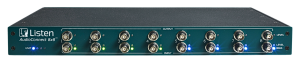
    The AudioConnect 8×8 audio interface is designed for accurate measurement in high channel-count applications. This high resolution interface offers 8 analog input and output channels plus 2 S/PDIF channels for digital signals. All input channels provide microphone power (constant voltage and constant current) and TEDS calibration support. Up to four AudioConnect 8×8’s can be connected for up to 32 synchronized analog input and output channels. AudioConnect 8×8 is fully configured via the software, making setup fast and easy, and allowing advanced features such as auto-ranging for maximum dynamic range measurements.


    2025:

  • 2025:


    Real Time Masking Curves Introduced

    SoundCheck is the first audio measurement software to offer real-time tonal masking and threshold-of-hearing curves in a spectrum analyzer. This demonstrates where a dominant tone is audibly masking other frequencies and noise to provide a clear visual correlation of measurements to audibility. When applied to a sound level spectrum measurement, the masking curves  automatically track the dominant tone, making any harmonics above the masking and threshold-of-hearing curves clearly visible. This simplifies diagnosis of the mechanisms causing the distortion.

  • 2024:

    Python Custom Step Introduced

    The Python custom step lets custom Python functions be called from a SoundCheck sequence, making it easy to pass data and variables between SoundCheck and other devices or programs, for example to send custom commands to put a device into diagnostic mode or to play a test signal from a device under test. It also enables communication with custom databases, and passing directional measurements to external programs.


    2024:

  • 2023:


    New Transient Distortion Algorithm - Enhanced Loose Particles

    Our enhanced Loose Particles algorithm brings a new level of accuracy and repeatability to transient distortion measurement, along with the ability to easily correlate measured results to audibility for easy limit setting. It uses the same time envelope analysis as our pioneering (2004) Loose Particles algorithm, but rather than filtering and counting pulses, additional analysis measures the prominence of the detected artifacts. This reflects the impulsiveness of the distortion more accurately than the absolute magnitude of the peaks. The algorithm allows the user to listen to the loose particle waveform with the stimulus removed, which enables easy correlation of the prominence threshold with audibility.


View Complete Timeline
https://www.listeninc.com/wp/media/2025/08/f-30logo-w.png 241 254 Zarina https://www.listeninc.com/wp/media/logo.png Zarina2025-08-10 16:59:052025-09-10 09:54:55Innovation Timeline – 30 Years
Page 4 of 31«‹23456›»

Audio Measurement Expertise


How Changing Industry Needs are Shaping Audio Test and Measurement

Smarter SoundCheck Sequences with Loops and Logic

Audio Basics: Polarity

How to Measure: Haptics

The Value of Big Data

Audio Basics: Phase Response

view all

Latest News


2026 End Of Year Promotions

Celebrating 30 years: Listening – The Secret Of Our Success

Automotive Test Sequence Including BSR, Max SPL and Frequency Response

Listen Introduces AudioConnect 2, a New Portable Dual-Channel Audio Interface

SoundCheck 21 Brings Enhanced Loose Particle Detection, Multichannel FFT, Metadata, Sequence Protection and more


Audio Measurement Expertise – Delivered Monthly


ABOUT LISTEN INC

Listen is a global leader in audio measurement and analysis, with over 30 years’ experience developing innovative test methods and algorithms. SoundCheck, our powerful software-based audio analyzer, pairs with our test interfaces, precision microphones, and accessories to offer a complete solution for testing loudspeakers, headphones, microphones, smart devices, communication systems, hearing aids, automotive audio, and more. Trusted by engineers worldwide, Listen delivers the accuracy and flexibility essential for modern audio testing, from the R&D lab to the production line.

PRODUCTS
APPLICATIONS
SUPPORT
RESOURCES
NEWS & EVENTS
ABOUT

CONNECT

YouTube
LinkedIn
LinkedIn
Share
Instagram

Copyright © Listen, Inc.   |   Privacy Policy   |   AI Disclosure
  • Instagram
  • LinkedIn
  • Youtube
  • Mail
Scroll to top