Want to measure your speaker at a specific SPL but not sure what voltage to use? In this video, we’ll show you how to calculate the exact test voltage needed to hit your target SPL using a simple SoundCheck sequence.
Additional Resources for SoundCheck
Detailed explanations of how to use SoundCheck can be found in the SoundCheck manual.
Video Transcript: Calculating Voltage for Target SPL
In an earlier video, I demonstrated how you can increment the test voltage level to see the frequency responses at various levels. But what if you want to run a speaker measurement at a specific sound pressure level and need to know what test voltage level to use?
I’ve written a short SoundCheck sequence to do this – let’s take a look.
First, the sequence asks the user to enter the desired target level in dB SPL. I’ll put 94dB as an example. It plays through a 1kHz sine tone and calculates the sensitivity, then implements a post-processing step to obtain the voltage level needed to output 94dB at 1kHz. The sequence then displays the calculated voltage level and the sensitivity level.
The rest of the sequence verifies this by running a stepped sine sweep using the calculated voltage level and outputting the frequency response. You will notice that at the 1kHz mark, it reflects the target level I input earlier, which is 94dB SPL.
This demo sequence can be downloaded from our website if you want to try incorporating it into your measurement sequences. Check it out, and if you have questions, please contact the Listen Support team.
https://www.listeninc.com/wp/media/2025/08/Calculating-Voltage-for-Target-SPL-Blog-TN.png10801080Julius Wijonohttps://www.listeninc.com/wp/media/logo.pngJulius Wijono2025-08-05 07:00:022026-08-27 14:10:26Calculating Voltage for Target SPL
In this second part of our car audio measurement demo, we’ll be covering how to measure maximum SPL at the onset of audible distortion and detect impulsive distortion using advanced SoundCheck sequences. You’ll see how to identify buzz, squeak, and rattle with perceptual Rub & Buzz, transient distortion, and crest factor analysis.
Watch this Video Demo of Car Audio Measurement Techniques
Learn More about How to Perform Car Audio Measurements
Video Transcript: How to Measure Car Audio – Part Two
Today, I’m going to continue on from our last automotive video where we measured frequency response, spectral uniformity, THD and IM distortion. This time we’ll demonstrate Max SPL at the onset of audible distortion and impulsive distortion. Let’s make some measurements.
Again, I’m using the test configuration recommended in the AES TC-AA white paper on automotive measurements. We’re using a precisely positioned 6-mic array in the driver’s seat to represent our listener. This is connected to an AmpConnect 621 Audio Interface. Our laptop is also connected to a measurement-grade Bluetooth interface which we’re using to send the stimulus signal into our car’s head unit. If you want to know more about the test configuration, you can download the AES white paper, and we also have full details on our website. The inputs and outputs of the test system are already calibrated, as is the audio interface, so we’re ready to measure.
Maximum SPL is one of themeasurements outlined in the TC-AA proposal, and it’s important because it lets you compare maximum sound levels of infotainment systems. It’s defined as the maximum sound pressure level that the infotainment system can reproduce, and it combines all the components of the system – the speakers, amplifiers, power supply and so on.
The simplest way of evaluating this is to measure the overall Max SPL and Max SPL spectrum regardless of distortion. In these tests we set the car’s volume control to maximum and measure overall Max SPL and SPL Spectrum simultaneously using a 30 second broadband 20 to 20 KHz monophonic pink noise stimulus at minus 12db FS . This is quite a basic measurement and I’ve demonstrated it in other videos, so we’ll just briefly discuss the results here, then I’ll demo a more advanced measurement.
Here we see the individual microphone measurements and the average, the black line. The overall level of 103dBC, regardless of distortion, isn’t too loud but maybe it might be limited by design to prevent severe distortion at low frequencies from clipping the amplifier.
What I’ll show you now is a Maximum SPL measurement at the onset of audible distortion. More volume is only good as long as the output sounds clean, so it makes sense to define the Maximum SPL based on when the sound quality starts to degrade.
This is a more complex test sequence and takes longer to run because you need to repeatedly play the stimulus until you reach distortion across a range of frequencies – similar to how we measure Max SPL in other applications. The good news is that this process can be highly automated in SoundCheck.
Our test sequence plays the stimulus multiple times for each test frequency, increasing the level in 3dB steps until the THD exceeds a predefined level in percent. It then reduces the level by 3dB and increases it in smaller increments of 0.5 dB to more precisely find the THD threshold. The Max SPL is recorded at that frequency and the test sequence continues to the next frequency. The entire process is completely automated via the test sequence, making this measurement fast with minimal intervention.
This sequence actually takes about 20 minutes to run in total, so I’ve edited this recording to skip the repetitive bits. We’ll set our range from 50 Hz up to 500 Hz, and we’ll set the percentage distortion. I’m going to set that at 3%. That means that once the distortion level goes above 3% it will record it and move onto the next frequency.
We’ll start at minus 12dB. The first thing it does is an auto range and it measures the time delay in the system… Now it’s playing 50 Hertz…It’s auto ranging. In a moment, it’s going to show the first result.
All right, here we go.
So, we can see the 50 Hertz sine wave of the 6 microphones capturing it, and we can see that we’re around 3.4% distortion.
So now it’s going to lower by 3 dB.
And it’s going to start going up again.
So now we’re 114 dB at 2.4%.
Now it’s going in half DB steps to very precisely find the sound pressure level at exactly 3%.
I’m just going to skip quickly through the next few measurements until we start graphing results
OK. We got 50, 63, and 80 Hz. You can see on the bottom graph is the input level and on the top graph we have the maximum sound pressure level versus frequency, the blue curve, and the orange curve is the THD level for that sound pressure level.
Again, I’ll fast-forward through the rest until we get our end result – it’s just more of the same at a bunch of different frequencies
OK, here’s our final result. The top graph shows the Maximum SPL and corresponding THD, and the lower graph shows the maximum stimulus level plotted when the THD reaches 3% with the head units’ volume control set to max.
At some frequencies, especially higher frequencies, for example 400 Hz and 500 Hz, the maximum input level is reached before the system distortion reaches 3% THD. The stimulus level is typically limited by the lower frequencies where there is more distortion.
So that’s it for system performance measurements. Now let’s look at system integrity.
Impulsive Distortion is a useful system integrity metric. It detects any audible buzz, squeak and rattle that may be caused by the speakers vibrating the door panels, loose wire harnesses, etc. These noises degrade the listener experience so it’s important to assess the vehicle thoroughly. It’s actually a good idea to make these measurements before you make the system characterization measurements, as this ensures that the infotainment system is properly installed in the vehicle under test
You can also use this test as an end-of-line check to verify vehicle integrity.
There are several methods of measuring impulsive distortion. The AES White Paper suggests a crest factor measurement with a logarithmic sine sweep and a tracking high pass filter, to evaluate impulsive distortion at 80 and 90 dBA. Sine waves have a crest factor of 3dB, and transients, such as rattling wires, loose fasteners, and noise, for example background noise, typically have a crest factor greater than 8dB. Generally speaking, crest factors over 3 dB, may indicate buzz, squeak or rattle. However, you have to be a bit careful as background noise, especially in a noisy factory, can result in similar Crest Factor results. You have to be very careful to minimize background noise and make sure that the results correlate with what you can hear.
I prefer to use perceptual Rub & Buzz and Transient distortion versus time instead, as they are less sensitive to background noise, and only highlight distortion sounds that are audible to humans. Perceptual Rub & Buzz uses masking curves to simulate the performance of the human ear to measure only audible distortion. Transient distortion versus time measurement tracks individual events in the time domain to reveal any loose particles or rattling wires. It offers greater precision than frequency domain measurements since it tracks individual transient events.
I’ll measure both these parameters simultaneously, using a stepped sine sweep stimulus.
There’s a couple of frequencies there where I could hear some buzzing or rattling sound, I’m not sure if you could hear it. Let’s see if we pick that up in the measurement.
OK, so here’s our recorded time waveform of all 6 mics.
And here… we can see the perceptual rub and buzz and indeed there’s a little bit of a peak going on at around 224 Hz and probably at a higher frequency here to around 340 Hz. These are the little buzzing sounds that we heard during the sweep.
Now, if we go to the bottom waveform graph, we can actually see if there’s any transients. Those are typically caused by things rattling around.
We don’t have much here – at low frequencies we don’t have a lot of output, so I suspect this is just background noise. So this car isn’t bad – just a little bit of Rub & Buzz and no transient artifacts.
I actually tried cranking the SPL up to 90dB to try to get some distortion at higher volumes, and here’s what I got…
Let’s just take a listen to the recorded response…. At this volume you can hear the distortion a lot more clearly.
Here we have the results of crest factor, Perceptual Rub & buzz and transient distortion.
The distortion is so obvious at this volume that it even shows up on the Crest Factor response – you can see the Crest Factor is above 8dB between 200 – 300 Hz.
It’s also much more obvious on the PRB curve – you can see a peak in the same point showing it correlates well. This is a little more sensitive than crest factor though – we can also see a smaller, sharper bump at 600 Hz which is not perceptible using crest factor measurement, even though I could hear it during the sweep. This measurement technique is also considerably more reliable in a noisy environment.
This 3rd graph shows the time transients of the impulsive distortion measurement. You can see the constant background noise as a steady noise floor and impulsive distortion is highlighted as well-defined transient spikes. You can see transient spikes from 2 of the microphones around 11-12 seconds into the sweep. These are closer to the driver side door where a door panel is rattling at low frequencies, around 200-300 Hz, in the sine sweep. A neat trick with this measurement method is that you can actually listen to the recording without the fundamental, let me just play that back now… and that really highlights the audible distortion.
So that pretty much concludes our suite of measurements. There are of course many variations of these measurements as well as other things you could measure with the same physical hardware setup, but that’s all we have time for today. There are some more in-depth automotive audio testing videos on our website and YouTube channel, so if you want to learn more, check them out.
https://www.listeninc.com/wp/media/2025/07/Car-Audio-Demo-Part-Two-TN-scaled.png14402560Julius Wijonohttps://www.listeninc.com/wp/media/logo.pngJulius Wijono2025-07-29 07:00:262026-08-28 14:26:17Car Audio Measurement – Part Two
Discover how masking curves in SoundCheck 23 bring psychoacoustics into your measurements with real-time tonal masking and threshold of hearing visualization – an industry first. In this video, we’ll show you how to use this new feature for production failure analysis and R&D insights by correlating what you see with what you hear.
Additional Resources for SoundCheck
Detailed explanations of how to use SoundCheck can be found in the SoundCheck manual.
Video Transcript: Using Masking Curves for Measurement Insights
A great new feature in SoundCheck 23 is the introduction of real-time tonal masking and threshold of hearing curves in the spectrum analyzer—an industry first. This lets you visualize how a dominant tone audibly masks other frequencies for a visual correlation between what we measure and what we hear. Let’s take a look at how to use it.
In production, it can give a deeper insight into failure analysis. Here, I have a small micro speaker. These designs are notorious for having rub and buzz problems around resonance due to their single-point suspensions. Let’s run our test sequence and examine the results.
The upper XY graph shows the fundamental and the enhanced perceptual Rub & Buzz (EPRB) curve. There’s a strong EPRB component focused right around 600 Hz. In the lower XY graph, we’re plotting the EPRB curve along with the electrical impedance curve, and we can see a strong correlation between the defect and the resonant frequency of the loudspeaker. On the waveform graph, zoomed in around 600 Hz, we can clearly see how distorted the waveform is. Now, let’s use the masking curve tool to investigate this defect further. I’ll open up a saved virtual instrument configuration that contains a signal generator and the FFT analyzer – the two tools you need to use masking curves.
The test level in our sequence was 200 milliVolts, but I’ll start the signal generator at 70 milliVolts and 600 Hz. At this level, a couple of harmonics are visible. Now let’s add our masking curve. We’ll add a calculation and select “Masking Curve” from the dropdown list. Our calculation is now a masking curve. Its name is calculation one and our operand is the FFT1 live curve. Now on our graph we can see our fundamental tone, our masking curve, and we can see that harmonics 2 and 3 are well below the masking curve, suggesting they should be inaudible.
But now, watch what happens as we increase the test level. Around 150 mV is when perceptual Rub & Buzz really takes off. Now nearly all harmonics above the fifth up to the 20th or so are above the masking curve. Now when we bring this up to our final test level of 200 mV, nearly every harmonic up to the 30th is touching or above the masking curve, so we’d expect this to sound pretty bad. Let’s take a quick listen… and as we would expect, we can hear a lot of distortion.
Finally, I’m going to remove the cursor and increase the frequency up to the point where the measured EPRB in our sequence should drop down. It’s doing some averaging, lets wait for it to settle. Now we can see at 800 hertz things have calmed down quite a bit. There’s still some visible harmonics but they’re pretty much at or below the masking curve. Let’s take it up to a kilohertz, now all our harmonics are below the masking curve and we should have a nice pure tone when we listen to it.
So there’s a look at how one might use this new feature for failure analysis on a production line. It also has R&D applications, such as monitoring the effects of component size and quality during product development—for example, the contributions of the voice coil and magnet system to harmonic distortion. To learn more, check out the SoundCheck manual.
https://www.listeninc.com/wp/media/2025/07/Masking-Curves-Blog-TN-1.png10801080Julius Wijonohttps://www.listeninc.com/wp/media/logo.pngJulius Wijono2025-07-22 07:00:342026-08-27 13:58:46Using Masking Curves for Measurement Insights
Everyone in audio test recognizes the ‘zip’ of the Stweep™, one of the world’s most ubiquitous audio test signals. But did you know it’s 30 years old this year?
It was developed by Steve Temme and made its debut in the first commercially available version of SoundCheck, launched in 1995. Since then, it has been adopted on thousands of production lines and in development labs worldwide and is still the stimulus of choice for testing a wide range of electroacoustic products, ranging from simple speaker drivers to complex automotive infotainment systems.
But what exactly is a ‘Stweep’, how is it different from a stepped sine sweep, and why has it stood the test of time so well?
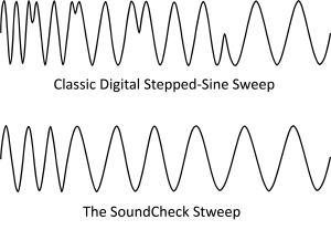
When you’re evaluating speakers, headphones, microphones, or other electroacoustic devices, the speed, accuracy, noise rejection and specific parameters that can be measured depend heavily on the stimulus signal used. Up until 1995, a standard stepped sine sweep was a popular choice for many electroacoustic tests as it produced results across a range of frequencies. This plays a sine wave at discrete frequencies, step by step, within a user-defined frequency range, and the user sets a resolution value to determine how many steps there will be.
Although extensively used, for example in the legendary Bruel and Kjaer 2012 analyzer, a stepped sine sweep has its limitations. It typically contains discontinuities because the frequencies do not change at a zero phase and amplitude crossing. This makes it slow as the device under test needs to settle at each new frequency. It is also inefficient at high frequencies where acoustic wavelengths are short, and potentially inadequate at low frequencies where settling times are long. The number of steps and their spacing are also critical. Too few steps can miss critical details; too many extend the test time unnecessarily.
In 1995 SoundCheck entered the market with the Stweep, a new proprietary test stimulus. The Stweep is an optimized stepped sine sweep that generates an integer number of cycles at each frequency step. This ensures a smooth “zero crossing” transition from step to step. It is also phase-continuous from frequency step to frequency step, which makes it sound more like a sine chirp than a stepped sine sweep. This reduces transducer ringing and decreases settling time which yields faster and more accurate measurements. Settling time is further reduced by sweeping from high to low as low frequencies have more energy than high frequencies.
The Stweep is user-configurable with different resolutions and averaging times at high and low frequencies to optimize the trade-off between stimulus duration and resolution. This customization enables a much faster sweep, cutting test time to a fraction of what it would be using the previous stepped sine method. As well as speed and accuracy, the Stweep demonstrates good noise immunity and allows many test parameters to be measured in parallel including frequency response, phase, harmonics, intermodulation with two sine waves, perceptual distortion metrics, and impedance,with a single sine sweep.
Over the past 30 years, the Stweep has become synonymous with fast, reliable end-of-line testing. It remains unmatched in its ability to combine acoustic, electrical, and perceptual measurements in a single sweep—delivering the speed, precision, and noise immunity modern production demands. A smoother continuous transition and other refinements introduced in 2017 further optimized its performance for large frequency steps and equalized measurements. While others are only now beginning to adopt similar stimuli, Listen’s Stweep continues to lead as one of the most advanced and versatile signals in the audio test engineer’s toolkit.
Traditional Stepped Sine Sweep
Stweep
https://www.listeninc.com/wp/media/2025/07/Sweep-vs-Stweep.png15722266Julius Wijonohttps://www.listeninc.com/wp/media/logo.pngJulius Wijono2025-07-18 10:22:572025-11-21 11:39:03Stweep Turns 30: The Test Signal That Changed Audio Measurement
Introducing AudioConnect 8×8, our latest audio interface engineered specifically for test and measurement applications. With 8 analog inputs and 8 outputs, expandable up to 32 in/32 out channels, this powerful, interface is ideal for audio test environments such as microphone arrays, loudspeaker directivity measurements, and automotive acoustic testing. It supports sample rates up to 192 kHz and offers built-in constant voltage and constant current power for a wide range of transducers, including SCM and IEPE microphones, accelerometers, and couplers. This eliminates the need for external power supplies and simplifies your setup.In this video, we’ll demonstrate its key features: secure BNC connections, selectable input gain with overload indicators, TEDS support for faster calibration, input monitoring, and seamless integration with SoundCheck software. You’ll also see how its configuration can be locked into test sequences to ensure consistency across labs and production lines.With simple setup and calibration, and fast configuration across multiple stations, AudioConnect 8×8 brings accuracy, control, and scalability to your audio testing workflow. Watch now to see how it can optimize your setup and improve efficiency in both R&D and manufacturing environments.
Detailed explanations of how to use SoundCheck can be found in the SoundCheck manual.
Video Transcript: The NEW AudioConnect 8×8™ Audio Interface
AudioConnect 8 by 8 is our first 8 in, 8 out audio interface that can be expanded up to 32 in, 32 out channels. Like our other interfaces, it’s specifically designed for audio measurements, with a host of design features to simplify your measurements and optimize your performance.
Let’s take a look.
On the front here we have our 8 analog input and output channels. These support sample rates up to 192 kHz so it’s great for high-resolution measurements. BNC connectors are used for secure cable connection and there are no knobs or buttons on the front panel. All the inputs provide both constant voltage for our SCM microphones and constant current for IEPE microphones and accelerometers. This means you can directly connect a wide range of transducers – microphones, head and torso simulators, couplers, test heads etc. Because you don’t need an additional power supply, this saves money especially if you are using a lot of channels for microphone arrays. Each input channel has several selectable gain options from -20 to +30dB, and includes level and overload indicators to ensure you’re operating within the optimal dynamic range. TEDS support is also included, which speeds the transducer calibration setup.
One other thing that’s pretty nice about the inputs is that you can monitor any of them if you want to listen to the response signal. In SoundCheck, you can assign an output to any input, then you can connect a headphone or loudspeaker on that output to monitor it.
Now let’s take a look at the back. Here you’ll see two power options – either a regular 100 to 240V supply, or a 12V DC supply which means that you can power it from a car or power bank out in the field. There’s S/PDIF in and out for a digital signal – BNC connectors again – and a USB-C connection to the computer.
Here we have our expansion ports. These 4 connectors let us synchronize up to 4 AudioConnect 8x8s together for a total of up to 32 input and output channels. I can plug in these 3 units to my master unit here, connect the master unit to the computer, and now I have 32 synchronized channels, and this is something you can’t do with most other interfaces.
This feature is really useful if you’re making directivity measurement with a large microphone array, or measuring large speaker arrays, or even making automotive measurements with a large number of microphones or speakers.
You’ll notice there are no physical knobs or buttons on the unit. All the functionality is controlled by SoundCheck to eliminate the risk of accidental gain or configuration changes. If you configure the hardware as part of a test sequence, it can’t be changed without editing the sequence. This means if you’re sharing sequences within your organization or with manufacturing partners, you can be 100% sure all the audio interface settings are correct and the tests are run exactly to your specifications.
Like our other hardware, setup is quick and easy. All channels are internally routed, so the only external connection required is a single USB cable to your computer. The device is supplied fully-calibrated, and when it’s connected to SoundCheck, the software automatically reads the calibration data from the firmware. This ensures a fully calibrated signal path with no manual input of sensitivity (Vp) values. You can see here the interface also auto-populates the input channels with appropriate sampling rates. It can also read and apply TEDS data if your microphones or accelerometers provide that.
It’s also quick and easy to setup multiple production line stations. Once you’ve configured it once, you can copy that configuration and each computer will automatically recognize the specific device connected to it. This also makes it easy to replace interfaces without recalibrating the signal path.
To learn more, check out the full specs on our website, www.listeninc.com, or contact your local sales engineer or rep for an in-person demo or pricing.
https://www.listeninc.com/wp/media/2025/07/AudioConnect-8x8-TN.png10801920Julius Wijonohttps://www.listeninc.com/wp/media/logo.pngJulius Wijono2025-07-18 07:00:202026-08-28 14:27:38The NEW AudioConnect 8×8™ Audio Interface
Curious how to view frequency directly in the time domain? In this video, we demonstrate how to use SoundCheck’s new Stimulus Frequency Cursor to pinpoint the frequency of transient events on recorded waveforms.
Additional Resources for SoundCheck
Detailed explanations of how to use SoundCheck can be found in the SoundCheck manual.
Video Transcript: How to View Frequency in the Time Domain
Today, I’m going to show you how to use SoundCheck’s Stimulus Frequency Cursor. This is a new feature we introduced in SoundCheck 23 that lets you see the exact frequency of any transient event on a recorded time waveform.
This feature can be used with:
Frequency Stepped Sweeps/Stweeps
Frequency Log Sweep
Log Amplitude Sweep
Two-tone options
Intermodulation
Difference Frequency
Loose Particle and Enhanced Loose Particle Waveform and Time Envelopes
Here I have a short sequence I’ll use for demonstration purposes. The first part uses play and record acquisition and harmonic track analysis, and the second part recalls some enhanced loose particle waveforms.
Let’s start the sequence and take a look at our recorded time waveform. We can see in our table here that the record delay is 1.11 milliseconds and we can clearly see that down here in the waveform graph. Let’s expand this graph so we can look at this new feature.
Now one thing that’s important to know when you’re using this feature, is that delay compensation must be added to our waveform. If I try to enable the stimulus frequency cursor now, you can see that it’s grayed out.
So, I’ll just add delay compensation in our analysis step… you can see here on the delay tab there’s a new function called “output auto-delayed waveforms” so I’ll select this and apply. If you keep your eye on the memory list and you’ll see a new waveform appear with the name “auto delayed recorded time waveform”.
Let’s bring this over to our waveform graph, and we can see this has essentially moved the start
of the recorded time waveform to time equals zero. Let’s remove the original one. Now we’ve done that, I can drop my stimulus frequency cursor onto this recorded time waveform. We can now see that we have the time and magnitude coordinates for our auto-delayed waveform, and here we have the frequency value. You can see these values changing as I drag the cursor across the waveform.
Now let’s take a look at how we can use the stimulus frequency cursor with loose particle analysis. We’ll continue running the sequence and it’s going to recall a previously recorded time waveform and perform an enhanced loose particle analysis on it.
Here we’ve got the recorded time waveform and down below is the enhanced loose particle waveform.
Let’s add our stimulus frequency cursor to the enhanced loose particle waveform. You can see that it’s already enabled – that’s because by default the ELP waveform is already delay compensated so we can jump right in and enable our stimulus frequency cursor and see the readout here. I can also use some of the other cursor functions like snap to max to see where the largest transient is on the graph – it’s telling me it’s at 200 hertz. Again, I can drag the cursor and see the frequencies change… we can see just by looking at it that the largest concentration of loose particle transient events occurs between 132 hertz and 250 hertz so that might help us understand a little bit more about the behavior of the loudspeaker.
So, that’s how we use the stimulus frequency cursor. If you want to learn more about this feature, check out the SoundCheck manual, or ask your sales engineer.
https://www.listeninc.com/wp/media/2025/07/Frequency-Time-Domain-Blog-TN.png10801080Julius Wijonohttps://www.listeninc.com/wp/media/logo.pngJulius Wijono2025-07-08 11:44:392026-08-27 14:22:14How to View Frequency in the Time Domain
Making accurate audio measurements in cars is complex and ever-changing as manufacturers incorporate functionality such as spatial audio, sound zones, vibration exciters, and more. Automotive companies, infotainment system subcontractors, consultants, and speaker manufacturers range from extensively testing every aspect of the system to measuring nothing at all. This article, originally published in the June 2025 issue of AudioXpress, discusses how the test configuration proposed by the TC-AA for three basic in-car measurements can also be used for a much larger suite of analyses.
The Audio Engineering Society (AES) Technical Committee on Automotive Audio published a white paper in 2023 proposing a standardized measurement configuration for in-car audio systems. This proposal covered three basic measurements: frequency response, Max SPL, and impulsive distortion. However as manufacturers add more complex audio to their cars, more sophisticated acoustic, vibration, electrical, and psychoacoustic measurements are needed.
Many of these measurements can be made with the same equipment configuration recommended by the TC-AA, enabling manufacturers to expand their portfolio of tests to match their precise needs and more completely characterize their audio performance. In this article, Steve Temme demonstrates some of these measurements including:
Seat-to-Seat Spectral Uniformity
Total Harmonic Distortion (THD)
Intermodulation Distortion (IMD)
Maximum SPL (Sound Pressure Level) at a fixed distortion percentage (e.g., 10% THD)
Impulsive Distortion using perceptual methods
These measurements provide a deeper understanding of audio system performance and help correlate results to human perception of sound inside a vehicle.
Explore how to automatically increment signal test levels using SoundCheck’s loop functionality. This technique is perfect for displaying measurements across a range of signal test levels, determining voltage-to-SPL relationships, or assessing distortion once a target level is reached.
Additional Resources for SoundCheck
Detailed explanations of how to use SoundCheck can be found in the SoundCheck manual.
Video Transcript: Auto-incrementing Signal Test Levels in SoundCheck
SoundCheck’s loop functionality offers a lot of flexibility, for example you can use it with sequence logic for pass/fail or yes/no scenarios, or to run tests in a loop and perform statistical analysis.
However, one of my favorite applications of this feature is for auto-incrementing the test signal level. This is useful, for example, to display measurements across different test signal levels, to ascertain the voltage required to achieve a specific sound pressure level or to measure distortion of a device once a desired sound pressure level is achieved.
In SoundCheck, when you create a loop, a memory list value called “loop index” is created and the steps are indented in the sequence editor.
In the step configuration window we can control the level at which the tests starts, and the increment amount. Here, I’ve set it to start at 100mV and increment in 100mV steps. This loop runs a total of 5 times and I have a table to reflect the test level for each cycle.
Now, let’s make sure our stimulus is using our incremental level. Open the stimulus step, and select “Memory List Selection” in the “level” section. Click on the dropdown and navigate to “loop index”, and change the axis to the Y-axis selection. You may get a prompt after doing this to disable the preload stimulus when using a memory list selection to control your test level. We do this by unchecking the “Preload Stimulus” option in the “Overall Sequence” configuration.
Now let’s run the sequence…
This table here displays the test level at every loop and our frequency responses, THD measurements, and recorded time waveforms are displayed for all 5 test runs.
Check it out, and if you have questions, please contact the Listen Support team.
https://www.listeninc.com/wp/media/2025/06/Signal-Test-Levels-Blog-TN.png10801080Julius Wijonohttps://www.listeninc.com/wp/media/logo.pngJulius Wijono2025-06-24 05:00:222026-08-27 14:18:19Auto-incrementing Signal Test Levels in SoundCheck
Check out our short demo video for a brief introduction to all the new features in SoundCheck 23. From real-time masking curves and multichannel oscilloscope support to ISO 532-3 loudness measurements and enhanced sequence editing, this release is packed with powerful features for both R&D and production.
SoundCheck 23 New Features
Ready to try SoundCheck 23 for yourself?
If you are ready to upgrade your system to SoundCheck 23, or want to discuss how SoundCheck 23 can help your testing needs, contact your local sales engineer or sales@listeninc.com with any questions.
Learn more
Download the PDF for SoundCheck 23 New Features here.
To see some of the other great features, algorithms, and functionality from previous SoundCheck versions, check out our version timeline to learn more about Listen’s 20 years of innovation.
SoundCheck 23 New Features Intro
Hello, I’m Steve Temme and today I’m going to demonstrate the new features in SoundCheck 23. This release is a big one for us as this year marks our 30th anniversary. When I created the first version of SoundCheck from the corner of my bedroom back in 1995, I had no idea that it would evolve into such a sophisticated audio test toolkit, or that some of those early algorithms I developed would go on to become industry standard test methods.
This new release offers new functionality and performance improvements for both R&D and production testing. These include real-time tonal masking curves for detailed perceptual audio analysis, a new multi-channel oscilloscope, a new time/ frequency cursor for recorded Stweep waveforms, and support for AudioConnect 8×8, our newest multi-channel interface. We’ve also improved performance, particularly for graphical display, and updated the sequence editor for faster test development. Let’s take a look.
https://www.listeninc.com/wp/media/2025/06/New-Features-Thumbnail-1.png10801920Julius Wijonohttps://www.listeninc.com/wp/media/logo.pngJulius Wijono2025-06-18 15:33:062026-08-21 12:34:27SoundCheck 23 New Features
How do you measure car audio? In this video, we demonstrate a complete car audio measurement setup using SoundCheck, based on the AES TC-AA recommended configuration. You’ll see how to test automotive infotainment systems inside a real vehicle using a calibrated 6-microphone array in the driver’s seat to capture spatially averaged data. We walk through measurements for frequency response (using both correlated and uncorrelated pink noise), seat-to-seat spectral uniformity, total harmonic distortion (THD), and intermodulation distortion.
Watch this Video Demo of Car Audio Measurement Techniques
Learn More about How to Perform Car Audio Measurements
Video Transcript: How to Measure Car Audio – Part One
Today I’m going to demonstrate in-car audio measurements, specifically frequency response, spectral uniformity and THD, using the test configuration recommended in the AES TC-AA white paper on automotive measurements.
We’re using a precisely positioned 6-mic array in the driver’s seat to represent our listener. This is connected to an AmpConnect 621 Audio Interface. Our laptop is also connected to a measurement-grade Bluetooth interface which we’re using to send the stimulus signal into our car’s head unit. If you want to know more about the test configuration, you can download the AES white paper, and we also have full details on our website.
I’ve already calibrated the inputs and outputs of the test system by measuring the sensitivity of each individual microphone in the array and storing these readings in the software calibration menu. I also calibrated the audio interface to ensure proper response frequencies and levels, both in the analog and digital domains, so we’re ready to measure.
First we’ll measure frequency response using 80 dBA monophonic, correlated, pink noise on both channels. I’ve already calibrated the level, and we’ll play a short burst. Ideally the stimulus should be longer but I’ll still get a pretty accurate result. Let’s start the sequence. Enter the information it’s asking. OK, the overall level is 79.5 dB, quite close to 80, with a delay of 1.45 seconds which SoundCheck has measured and compensated for. What I’ve actually done here is a 1/3 octave analysis of each individual microphone, from 1 through 6, and you can see the difference due to location, reflections, and standing waves in the car. The black curve is the overall power average or spatial average of all six mics and represents what a human would hear.
Now let’s measure the frequency response using uncorrelated pink noise. This randomizes the noise between the two channels rather than playing identical signals out of both. We expect to see some low frequency cancellation due to phase differences.
So let’s run the sequence… and we’ve got our results.
We can compare the results with uncorrelated noise to the results when I used correlated pink noise. Let’s bring them both onto the graph… The orange line is the correlated spatial average and the black line is the uncorrelated spatial average. We can see the uncorrelated pink noise has about 3db less output than the correlated pink noise below 100 Hz and very little above 1KHz.
We can also look at the seat to seat spectral uniformity. Ideally each passenger in the car experiences the same high quality sound, but it’s hard to independently equalize the loudspeaker playback system for each seat in the car. Typically the driver’s seat is favored, the frequency response in the other seats is not quite as smooth.
I’m not going to do this now as it takes a while, but I’ll show you some measurements I made earlier. I repeated the first frequency response measurement with correlated pink noise in each of the car’s four seats and here you can see that the base performance in the rear passenger seats, the orange and green lines are not as extended or smooth as the front passenger seats.
To calculate the seat to seat spectral uniformity, We compare the individual seat response to the maximum and minimum responses to find the seat with the biggest difference. In this example both the left and right rear passenger seats have over 10 dB difference from the front seats at some
Frequencies. The lower the number the more uniform the frequency response is from seat to seat.
Now let’s make some distortion measurements. We’ll start with THD.
THD indicates the overall nonlinear performance of the device, and if it’s outside the limits it might indicate a poorly centered voice coil or mechanical defects. We measure total harmonic Distortion at 80 dBA, this time using a stepped sign sweep from high to low with 12th octave steps.
Let’s run it… As before, we power sum the spatial average of all six microphones to produce the THD power average curve, this black line here, which smooths out the standing waves and reflections picked up by the individual microphones. That’s not too bad – if we look at the power average we’re getting roughly 2.2% from 50 to 10 kHz.
Next we’ll look at intermodulation Distortion. This is a good test for multi-way speaker systems with a crossover- if a small driver is trying to play back low and high frequencies simultaneously it’ll struggle to play both frequencies and create IM distortion. Here we use a two-tone stimulus with a fixed tone set to 50Hz, and a sweep tone that sweeps high to low from 20 kHz down to 150 Hz. I’ve already run a couple of sweeps to set the auto delay and to Auto Range the input gain for the best signal to noise ratio – this is important to ensure that the harmonics are above the noise floor of the measurement. Now let’s start the measurement.
OK… The graph shows the fundamental and total Intermodulation Distortion of the second and third order intermodulation products, power averaged from the six microphone array. As you might expect, there’s more IM distortion at the lower frequencies, but you can see an increase around 700 Hz – that’s probably a crossover frequency in this car. If we take the spatial average of all six mics we get an overall IM distortion level of 1.4%.
That’s all we have time for here – check out part 2 for Max SPL and more distortion measurements!
https://www.listeninc.com/wp/media/2025/06/Car-Audio-Demo-Part-One-TN.png10801920Julius Wijonohttps://www.listeninc.com/wp/media/logo.pngJulius Wijono2025-06-16 14:19:532026-08-28 14:23:23Car Audio Measurement – Part One


 Everyone in audio test recognizes the ‘zip’ of the Stweep™


 Making accurate audio measurements in cars is complex and ever-changing as manufacturers incorporate functionality such as spatial audio, sound zones, vibration exciters, and more. Automotive companies, infotainment system subcontractors, consultants, and speaker manufacturers range from extensively testing every aspect of the system to measuring nothing at all. This article, originally published in the June 2025 issue of AudioXpress, discusses how the test configuration proposed by the TC-AA for three basic in-car measurements can also be used for a much larger suite of analyses.


